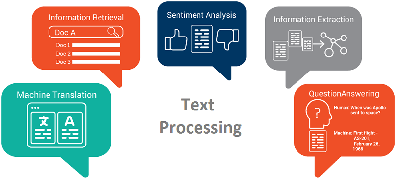
Text Processing is one of the most common task in many ML applications. Below are some examples of such applications.
• Language Translation: Translation of a sentence from one language to another.
• Sentiment Analysis: To determine, from a text corpus, whether the sentiment towards any topic or product etc. is positive, negative, or neutral.
• Spam Filtering: Detect unsolicited and unwanted email/messages.
These applications deal with huge amount of text to perform classification or translation and involves a lot of work on the back end. Transforming text into something an algorithm can digest is a complicated process. In this article, we will discuss the steps involved in text processing.
Step 1 : Data Preprocessing
- Tokenization — convert sentences to words
- Removing unnecessary punctuation, tags
- Removing stop words — frequent words such as ”the”, ”is”, etc. that do not have specific semantic
- Stemming — words are reduced to a root by removing inflection through dropping unnecessary characters, usually a suffix.
- Lemmatization — Another approach to remove inflection by determining the part of speech and utilizing detailed database of the language.
The stemmed form of studies is: studi
The stemmed form of studying is: study
The lemmatized form of studies is: study
The lemmatized form of studying is: study
Thus stemming & lemmatization help reduce words like ‘studies’, ‘studying’ to a common base form or root word ‘study’. For detailed discussion on Stemming & Lemmatization refer here . Note that not all the steps are mandatory and is based on the application use case. For Spam Filtering we may follow all the above steps but may not for language translation problem.
We can use python to do many text preprocessing operations.
- NLTK — The Natural Language ToolKit is one of the best-known and most-used NLP libraries, useful for all sorts of tasks from t tokenization, stemming, tagging, parsing, and beyond
- BeautifulSoup — Library for extracting data from HTML and XML documents
#using NLTK library, we can do lot of text preprocesing
import nltk
from nltk.tokenize import word_tokenize
#function to split text into word
tokens = word_tokenize("The quick brown fox jumps over the lazy dog")
nltk.download('stopwords')
print(tokens)
OUT: [‘The’, ‘quick’, ‘brown’, ‘fox’, ‘jumps’, ‘over’, ‘the’, ‘lazy’, ‘dog’]
from nltk.corpus import stopwords
stop_words = set(stopwords.words(‘english’))
tokens = [w for w in tokens if not w in stop_words]
print(tokens)
OUT: [‘The’, ‘quick’, ‘brown’, ‘fox’, ‘jumps’, ‘lazy’, ‘dog’]
#NLTK provides several stemmer interfaces like Porter stemmer, #Lancaster Stemmer, Snowball Stemmer
from nltk.stem.porter import PorterStemmer
porter = PorterStemmer()
stems = []
for t in tokens:
    stems.append(porter.stem(t))
print(stems)
OUT: [‘the’, ‘quick’, ‘brown’, ‘fox’, ‘jump’, ‘lazi’, ‘dog’]
Step 2: Feature Extraction
In text processing, words of the text represent discrete, categorical features. How do we encode such data in a way which is ready to be used by the algorithms? The mapping from textual data to real valued vectors is called feature extraction. One of the simplest techniques to numerically represent text is Bag of Words.
Bag of Words (BOW): We make the list of unique words in the text corpus called vocabulary. Then we can represent each sentence or document as a vector with each word represented as 1 for present and 0 for absent from the vocabulary. Another representation can be count the number of times each word appears in a document. The most popular approach is using the Term Frequency-Inverse Document Frequency (TF-IDF) technique.
- Term Frequency (TF) = (Number of times term t appears in a document)/(Number of terms in the document)
- Inverse Document Frequency (IDF) = log(N/n), where, N is the number of documents and n is the number of documents a term t has appeared in. The IDF of a rare word is high, whereas the IDF of a frequent word is likely to be low. Thus having the effect of highlighting words that are distinct.
- We calculate TF-IDF value of a term as = TF * IDF
Let us take an example to calculate TF-IDF of a term in a document.
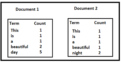
TF('beautiful',Document1) = 2/10, IDF('beautiful')=log(2/2) = 0
TF(‘day’,Document1) = 5/10,  IDF(‘day’)=log(2/1) = 0.30

TF-IDF(‘beautiful’, Document1) = (2/10)*0 = 0
TF-IDF(‘day’, Document1) = (5/10)*0.30 = 0.15
As, you can see for Document1 , TF-IDF method heavily penalizes the word ‘beautiful’ but assigns greater weight to ‘day’. This is due to IDF part, which gives more weightage to the words that are distinct. In other words, ‘day’ is an important word for Document1 from the context of the entire corpus. Python scikit-learn library provides efficient tools for text data mining and provides functions to calculate TF-IDF of text vocabulary given a text corpus.
One of the major disadvantages of using BOW is that it discards word order thereby ignoring the context and in turn meaning of words in the document. For natural language processing (NLP) maintaining the context of the words is of utmost importance. To solve this problem we use another approach called Word Embedding.
Word Embedding: It is a representation of text where words that have the same meaning have a similar representation. In other words it represents words in a coordinate system where related words, based on a corpus of relationships, are placed closer together.
Let us discuss some of the well known models of word embedding:
Word2Vec
Word2vec takes as its input a large corpus of text and produces a vector space with each unique word being assigned a corresponding vector in the space. Word vectors are positioned in the vector space such that words that share common contexts in the corpus are located in close proximity to one another in the space. Word2Vec is very famous at capturing meaning and demonstrating it on tasks like calculating analogy questions of the form a is to b as c is to ?. For example, man is to woman as uncle is to ? (aunt) using a simple vector offset method based on cosine distance. For example, here are vector offsets for three word pairs illustrating the gender relation:
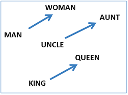
This kind of vector composition also lets us answer “King — Man + Woman = ?” question and arrive at the result “Queen” ! All of which is truly remarkable when you think that all of this knowledge simply comes from looking at lots of word in context with no other information provided about their semantics. For more details refer here.
Glove
The Global Vectors for Word Representation, or GloVe, algorithm is an extension to the word2vec method for efficiently learning word vectors. GloVe constructs an explicit word-context or word co-occurrence matrix using statistics across the whole text corpus. The result is a learning model that may result in generally better word embeddings.
Consider the following example:
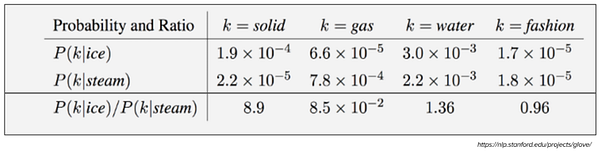
Target words: ice, steam
Probe words: solid, gas, water, fashion
Let P(k|w) be the probability that the word k appears in the context of word w. Consider a word strongly related to ice, but not to steam, such as solid. P(solid | ice) will be relatively high, and P(solid | steam) will be relatively low. Thus the ratio of P(solid | ice) / P(solid | steam) will be large. If we take a word such as gas that is related to steam but not to ice, the ratio of P(gas | ice) / P(gas | steam) will instead be small. For a word related to both ice and steam, such as water we expect the ratio to be close to one. Refer here for more details.
Word embeddings encode each word into a vector that captures some sort of relation and similarity between words within the text corpus. This means even the variations of words like case, spelling, punctuation, and so on will be automatically learned. In turn, this can mean that some of the text cleaning steps described above may no longer be required.
Step 3: Choosing ML Algorithms
There are various approaches to building ML models for various text based applications depending on what is the problem space and data available.
Classical ML approaches like ‘Naive Bayes’ or ‘Support Vector Machines’ for spam filtering has been widely used. Deep learning techniques are giving better results for NLP problems like sentiment analysis and language translation. Deep learning models are very slow to train and it has been seen that for simple text classification problems classical ML approaches as well give similar results with quicker training time.
Let us build a Sentiment Analyzer over the IMDB movie review dataset using the techniques discussed so far.
Download the IMDb Movie Review Data
The IMDB movie review set can be downloaded from here. This dataset for binary sentiment classification contains set of 25,000 highly polar movie reviews for training, and 25,000 for testing. This dataset was used for the very popular paper ‘Learning Word Vectors for Sentiment Analysis’.
Preprocessing
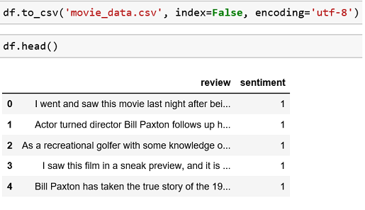
The dataset is structured as test set and training set of 25000 files each. Let us first read the files into a python dataframe for further processing and visualization. The test and training set are further divided into 12500 ‘positive’ and ‘negative’ reviews each. We read each file and label negative review as ‘0’ and positive review as ‘1’
#convert the dataset from files to a python DataFrame
import pandas as pd
import os
folder = 'aclImdb'
labels = {'pos': 1, 'neg': 0}
df = pd.DataFrame()
for f in ('test', 'train'):
    for l in ('pos', 'neg'):
        path = os.path.join(folder, f, l)
        for file in os.listdir (path) :
            with open(os.path.join(path, file),'r', encoding='utf-8') as infile:
                txt = infile.read()
            df = df.append([[txt, labels[l]]],ignore_index=True)
df.columns = ['review', 'sentiment']
Let us save the assembled data as .csv file for further use.
To get the frequency distribution of the words in the text, we can utilize the nltk.FreqDist() function, which lists the top words used in the text, providing a rough idea of the main topic in the text data, as shown in the following code:
import nltk
from nltk.tokenize import word_tokenize
reviews = df.review.str.cat(sep=' ')
#function to split text into word
tokens = word_tokenize(reviews)
vocabulary = set(tokens)
print(len(vocabulary))
frequency_dist = nltk.FreqDist(tokens)
sorted(frequency_dist,key=frequency_dist.__getitem__, reverse=True)[0:50]
This gives the top 50 words used in the text, though it is obvious that some of the stop words, such as the, frequently occur in the English language.

Look closely and you find lot of unnecessary punctuation and tags. By excluding single and two letter words the stop words like the, this, and, that take the top slot in the word frequency distribution plot shown below.
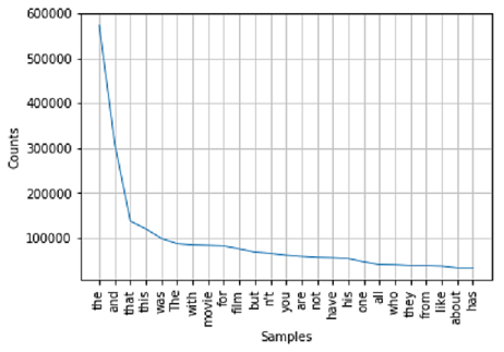
Let us remove the stop words to further cleanup the text corpus.
from nltk.corpus import stopwords
stop_words = set(stopwords.words('english'))
tokens = [w for w in tokens if not w in stop_words]

This looks like a cleaned text corpus now and words like went, saw, movieetc. taking the top slots as expected.
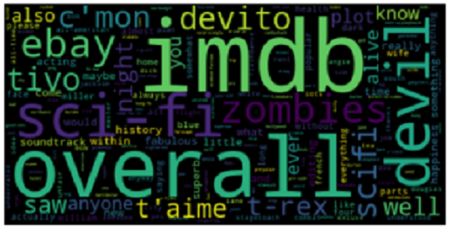
Another helpful visualization tool wordcloud package helps to create word clouds by placing words on a canvas randomly, with sizes proportional to their frequency in the text.
from wordcloud import WordCloud
import matplotlib.pyplot as plt
wordcloud = WordCloud().
generate_from_frequencies(frequency_dist)
plt.imshow(wordcloud)
plt.axis("off")
plt.show()
Building a Classifier
After cleanup, it is time to build the classifier to identify sentiment of each movie review. From the IMDb dataset, divide test and training sets of 25000 each:
X_train = df.loc[:24999, 'review'].values
y_train = df.loc[:24999, 'sentiment'].values
X_test = df.loc[25000:, 'review'].values
y_test = df.loc[25000:, 'sentiment'].values
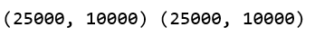
We use TfidTransformer to covert the text corpus into the feature vectors, we restrict the maximum features to 10000. For further details about how to useTfidTransformerrefer here.
from sklearn.feature_extraction.text import TfidfTransformer
from sklearn.feature_extraction.text import TfidfVectorizer
vectorizer = TfidfVectorizer()
train_vectors = vectorizer.fit_transform(X_train)
test_vectors = vectorizer.transform(X_test)
print(train_vectors.shape, test_vectors.shape)
There are many algorithms to choose from, we will use a basic Naive Bayes Classifier and train the model on the training set.
from sklearn.naive_bayes import MultinomialNB
clf = MultinomialNB().fit(train_vectors, y_train)
Our Sentiment Analyzer is ready and trained. Now let us test the performance of our model on the test set to predict the sentiment labels.
from sklearn.metrics import accuracy_score
predicted = clf.predict(test_vectors)
print(accuracy_score(y_test,predicted))
Output 0.791
Wow!!! Basic NB classifier based Sentiment Analyzer does well to give around 79% accuracy. You can try changing features vector length and varying parameters ofTfidTransformerto see the impact on the accuracy of the model.
Conclusion: We have discussed the text processing techniques used in NLP in detail. We also demonstrated the use of text processing and build a Sentiment Analyzer with classical ML approach achieved fairly good results.
Thanks for reading this article, recommend and share if you like it.